3 Preparation
3.1 Explore data
3.1.1 Checking the sampling rate
summarize_sampling_rate_many(tar_read(tracks), 'id')| id | min | q1 | median | mean | q3 | max | sd | n | unit |
|---|---|---|---|---|---|---|---|---|---|
| 1072 | 3.92 | 9.8 | 10.0 | 20.7 | 10.3 | 1650 | 95 | 1348 | min |
| 1465 | 0.40 | 2.0 | 2.0 | 8.9 | 4.0 | 1080 | 48 | 3003 | min |
| 1466 | 0.42 | 2.0 | 2.1 | 15.7 | 4.1 | 2167 | 104 | 1500 | min |
| 1078 | 1.35 | 9.8 | 10.0 | 21.7 | 10.3 | 2111 | 87 | 1637 | min |
| 1469 | 0.42 | 2.0 | 2.2 | 13.2 | 5.4 | 2889 | 90 | 2435 | min |
| 1016 | 0.07 | 1.9 | 2.0 | 8.0 | 2.5 | 1209 | 44 | 8957 | min |
3.2 Clean data
3.2.1 Erroneous locations
The amt package includes code and guidelines for data cleaning, as does Bjørneraas et al. (2010).
The major GPS cleaning considerations are:
- censor locations pre- and post- animal capture and collaring
- low quality data (based on the available measure of precision, 2D/3D, DPOP, etc.)
- unreachable habitats to occupy
- unrealistic step lengths
- immediate round trips
- drop offs/ mortalities
3.2.2 Rarefication and Autocorrelation
In early GPS and RSF studies, autocorrelation was viewed as an issue to directly eliminate. Over the last two decades, however, the discourse around autocorrelation has become more nuanced (Fieberg et al. 2021; Northrup et al. 2022). To summarize our current understanding, locations are indeed ‘serially dependent’ – points closer in time will be closer in space (Fleming et al. 2014). However, if these locations are taken at regular intervals, they should be representative of space use (Fieberg et al. 2021). Sampling locations at regular intervals is the best practice for habitat selection analyses. Further, autocorrelation bias will reduce estimate of uncertainty (SE). To address concern, using a robust calculation for confidence intervals can be completed.
3.3 Sample Available Steps
The main assumption is that the availability distribution defines what is accessible to the animal at a given location or time. For SSF specifically this assumption addresses what is accessible to the animal and can be selected as it makes its next step.
iSSA builds on this and uses empirical observations of movements to inform probability distributions, which can then be modified by including corresponding covariates in the model.
The unit of replication in iSSA analysis are clusters (or strata) made of a used step matches with a set of available steps. Available steps are sampled from tentative distributions of step length and turn angle.
3.3.1 Distributions
Be aware what distribution you are drawing from when you generate random steps.
3.3.1.1 Step Length Distribution
There are four possible step length distributions:
- Exponential (step length)
- Half-Normal ([step-length]2)
- Log-Normal (log[step length]2 and log[step length]
- Gamma (step length and log[step length])
Here we will focus on the Gamma, as it has been commonly used in the literature,
but will provide some exponential examples. The Gamma distribution has a shape
(k) and a scale parameter (\(\theta\), ‘shape’ and ‘scale’ in the amt package. The
exponential distribution, which is a special case of the gamma, only has a rate
parameter (lambda).
tar_read(dist_sl_plots, 1)## $dist_sl_plots_8ba21cb0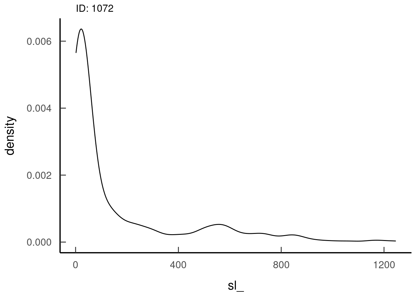
Plot the observed data against these fitted distributions to assess the agreement between them. Do the distributions misclassify some observations (normally will miss extreme values)? There should not be negative speeds at this point, calculate the mean to check. These plots and calculations should be done at the level you estimated distributions, calculated random steps, and model the behaviour. Check which distribution seems to fit best.
3.3.1.2 Turn Angle Distribution
Prokopenko et al. (2016) used a uniform ta and included cos(TA) to
adjust for more realistic variation in directionality. If a Von Mises is fit
from observed points, including cos(TA) in the model might not be informative.
The concentration parameter (k) ‘kappa’ in amt, and the location parameter
(\(\mu\), mu in amt).
tar_read(dist_ta_plots, 1)## $dist_ta_plots_8ba21cb0## Warning: Removed 35 rows containing non-finite values (stat_density).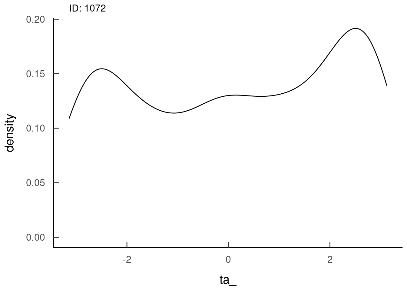
3.3.1.3 Individual vs. Population Distributions
When generating random steps for multiple animals, you can do so at either the
individual or population level distribution. When you generate random steps by
individuals, the amt package is fitting a parametric distribution to the step
length and turn angle distributions of a given individual and then randomly
selecting new steps from it.
As an alternative, the population level distribution can be used, which informs random steps for all individuals using this population probability distribution. You could also split movement distributions by time of day, or season, even by habitat.
How you generate random distributions changes your comparisons of used to
available. For example, if you generate distributions from the population and
run individual models. Then the results will say how individuals differ from the
population movement behaviour. Let’s consider a fast individual, if a population
SL distribution was used then their ln(SL) covariate will be more positive to
adjust for this different. If you want to compare individuals to each other,
then starting with a baseline that is the same allows you to do so, the
population mean distribution is recommended.
In summary, movement variation can be accounted for at the random step generation stage and/or in the model parameterization stage. There are reasons for either, but the awareness of which one you choose and possible downstream patterns that could result is critical.
These decisions can be informed once you explore your data.
3.3.2 Number of random steps
The availability distribution is defined by the randomly sampled steps from the step length and turn angle probability distributions.
Using 10 steps for each used step to have a strata of 11 steps is common, but intensity of sampling varies across the literature. Sensitivity analysis can be conducted to determine the influence of availability sample on selection (Northrup et al. 2013, 2016). A general piece of advice is “at least one, the more the merrier” (Avgar and Smith 2022)
Generating tracks:
make_track(locs_prep, x_, y_, t_, all_cols = TRUE, crs = epsg)Resampling tracks:
resample_tracks(tracks, rate = rate, tolerance = tolerance)Adding random steps:
random_steps(tracks_resampled, n = n_random_steps)Researchers should consider the resolution of the habitat covariate and the step length of the animal to determine the number of steps required to estimate what is accessible to the animal.
3.4 Explore data
3.4.1 Guiding Questions
- What is the sample size of the data going into the model?
- What are the data layer resolution and extent?
- How does this relate to your location data?
- How does movement vary within and between biological/ecological divisions?
The purpose of exploring your data is to brainstorm the potential options for your models and identify potential limitations. Proper exploration of used (case = 1) and available (case = 0) domains by individual, population, season, year etc. will help inform downstream decisions and troubleshoot convergence issues.
# > table or figure sample size - # individuals and points per individual
# > locations spread per season, year, individual: counts across categories
# > density or histogram or box plot of covariates for used and available by any division that might be used in the model individual, year, season
# > temporal extent and resolution
# > spatial extent and resolution
# > movement rates and turn angles by individual, season, time of day: mean, range, plots
3.5 Attribute steps
- End-point = selection processes
- Start-point = movement processes
Attributes extracted at the start-point do not vary within a cluster, but can be used as interactions with movement covariates or habitat-selection covariates (at the end point)
3.5.1 Choosing covariates
3.5.1.1 Guiding questions
- What are your research objectives and hypotheses?
- What are the data layers you need to meet these objectives and test these hypotheses?
- What are the data layer resolution and extent? How does this relate to your location data?
- Will continuous or categorical covariates best help your answer your research questions (and are there computational limitations to one or the other)?
3.5.2 Availability threshold
Dickie et al. (2020) used 0.01 as the “threshold” of availability. i.e. included the variable in the model if the available steps had at least 1% of that habitat type, and otherwise booted it out. I think the more typical choice would be 5%, Dickie was able to get reasonable estimates with most individuals fitting at 1%.
tar_read(avail_lc)[id == 1016]| id | prop_lc_description | lc_description |
|---|---|---|
| 1016 | 0.49 | forest |
| 1016 | 0.16 | developed |
| 1016 | 0.01 | shrubland |
| 1016 | 0.20 | wetlands |
| 1016 | 0.06 | cultivated |
| 1016 | 0.08 | water |
| 1016 | 0.00 | herbaceous |
Depending on how many covariates you have in your model, having many habitat classes (and any associated interactions) can really eat up your data. It’s worthwhile doing a habitat point extraction for your GPS locations to see which habitat types are relevant and available to your individuals. Then you can start to combine some habitat types. For example, open vs closed, deciduous vs coniferous vs mixed, etc.
3.5.3 Selection
Selection is represented by the end-point of a step, i.e., where an animal selects to be. The covariate of interest at the end point can be interacted with any other habitat metric from the preceding step or one that is also at the end-point.
- Data types: continuous, categorical, Boolean
Important: discrete variable must be coded as factors.
- Transforming and scaling covariates (GLMM TMB, same scale is critical for mixed model, still helpful in clogit models but less necessary)
The extract_layers function is a user-facing function from the
targets-issa workflow to flexibly sample relevant spatial layers.
In the example, it samples land cover (point), elevation (point),
population density (point), and water (distance to). It also
combines the merges the land cover legend to provide more useful
land cover descriptions in addition to numeric ids.
# R/extract_layers.R
extract_layers
function (DT, crs, lc, legend, elev, popdens, water)
{
setDT(DT)
start <- c("x1_", "y1_")
end <- c("x2_", "y2_")
extract_pt(DT, lc, end)
DT[legend, `:=`(lc_description, description), on = .(pt_lc = Value)]
extract_pt(DT, elev, end)
extract_pt(DT, popdens, end)
extract_distance_to(DT, water, end, crs)
}Scaling covariates
- will influence magnitude of coefficients, ideally scale of covariates will be within an order of magnitude.
- distance from features, likely should follow decay function (i.e.,
log-transformed). Note
log()in R is the natural logarithm, not log base 10.
3.5.4 Movement
To look at the influences of habitat on movement interact the covariate at the start of step with turn angle or step length. Possible movement covariates include step length, ln[step length], [step length]2, ln[step length]2,cos[turn angle].
3.5.5 Other Covariate Notes
3.5.5.1 Time of Day
Time of day will not vary between clusters. In our experience, ‘time of day’ has
narrow in the definition of twilight periods in amt package. amt::time_of_day
which is a wrapped around maptools::crepuscule. The potential underestimation
comes from default solarDep / solar.dep, which can be adjusted. This matters
especially for fix rates that are longer than the crepuscule period because
there may be a fix during that period or only 1, leading to the underestimation.
Identifying crepuscule movements may not matter to your analysis, in which case,
don’t include it when calculating time of day (crepuscule = FALSE). If you
need to include crepuscular movement, adjust the default solarDep or create
your own calculation (can link to Katrien’s or mine for wolves).
# > time of day3.5.5.2 Interactions
If you included interactions, then the model has an estimate for both terms independently and as well as the interaction. So interaction I:J will have betas for I, J, and I:J. If J is a category there will be estimates for each category. If there is a three way interact I:J:K, you get estimates for I,J,K, I:J, I:K, J:K, and I:J:K.
Before Running your Model: Check correlation between covariates
EXERCISE: Create a table of with each covariate and the corresponding
prediction or biological significance?
Example Table: prediction and covariates.