5 Interpretation
5.1 What’s in a beta?
- In iSSA they can pertain to either selection or movement behaviour. They indicate directionality but the ecological significance and effect size of the behaviour is not clear without predicting the model
5.1.1 Selection
- Coefficient for covariate indicates selection (+) or avoidance (-)
- “Distance-to a feature” covariate can be tricky, a positive coefficient indicates selection for areas farther from the feature, which means the feature itself is avoided.
5.1.2 Movement
- Coefficient for log(Step Length) modifies shape parameter indicating more (+) or fewer long steps (-)
- Coefficient for Step Length modifies the scale parameter indicating longer (+) or shorter steps (-)
- Coefficient for cos(Turn Angle) indicates the directionality of movement, concentration parameter of the Von Mises
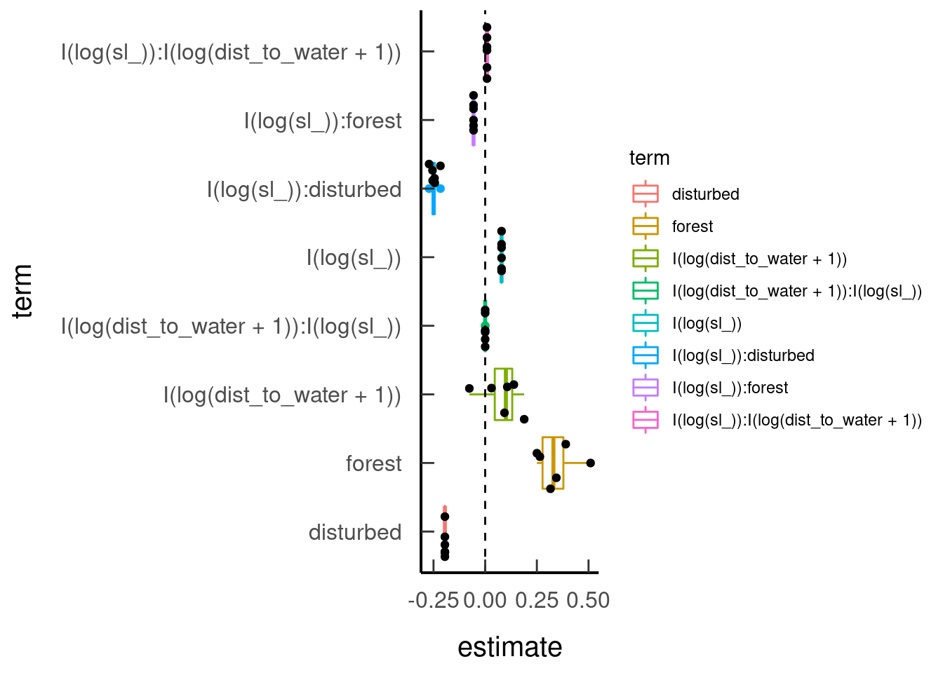
5.1.3 Presenting coefficients
5.1.3.1 Table
A table with coefficient and error is standard for reporting results. This is not recommended for presentations or the sole means of presenting results.
broom.mixed::tidy(tar_read(model_forest), effects = 'fixed')| effect | component | term | estimate | std.error | statistic | p.value |
|---|---|---|---|---|---|---|
| fixed | cond | I(log(sl_)) | 0.08 | 0.08 | 1.02 | 0.31 |
| fixed | cond | forest | 0.35 | 0.19 | 1.79 | 0.07 |
| fixed | cond | disturbed | -0.19 | 0.28 | -0.70 | 0.48 |
| fixed | cond | I(log(dist_to_water + 1)) | 0.08 | 0.09 | 0.92 | 0.36 |
| fixed | cond | I(log(sl_)):forest | -0.06 | 0.04 | -1.55 | 0.12 |
| fixed | cond | I(log(sl_)):disturbed | -0.25 | 0.05 | -4.65 | 0.00 |
| fixed | cond | I(log(sl_)):I(log(dist_to_water + 1)) | 0.01 | 0.01 | 0.77 | 0.44 |
5.2 Effect Sizes
We strongly advocate for going beyond presenting the coefficients and errors to demonstrate the effect sizes of response across the environmental variation.
5.2.1 Relative Selection Strength
Calculated for an animal selecting one spatial location (x1) over another (x2) when these two locations are the same except for one habitat covariate
- Common RSS expressions in Avgar et al. (2017), formulation depends on the covariates of interest in model
- Can use the
predictfunction: https://rdrr.io/cran/amt/man/log_rss.html in amt or JWT code (see Full workflow for an example) - Fieberg ‘How-to’ goes through the RSS maths (Fieberg et al. 2021)
In the targets-issa workflow, we predict H1, and H2 for forest using the following functions:
# R/predict_h1_water.R
predict_h1_water
function (DT, model)
{
N <- 100L
new_data <- DT[, .(sl_ = mean(sl_), forest = 0, disturbed = 0,
dist_to_water = seq(from = 0, to = 1500, length.out = N),
indiv_step_id = NA), by = id]
new_data[, `:=`(h1_water, predict(model, .SD, type = "link",
re.form = NULL))]
new_data[, `:=`(x, seq(from = 0, to = 1500, length.out = N)),
by = id]
}
# R/predict_h2.R
predict_h2
function (DT, model)
{
new_data <- DT[, .(sl_ = mean(sl_), forest = 0, disturbed = 0,
dist_to_water = median(dist_to_water, na.rm = TRUE),
indiv_step_id = NA), by = id]
new_data[, `:=`(h2, predict(model, .SD, type = "link", re.form = NULL))]
}Then we can calculate RSS for forest:
# R/calc_rss.R
calc_rss
function (pred_h1, h1_col, pred_h2, h2_col)
{
log_rss <- merge(pred_h1[, .SD, .SDcols = c("id", "x", h1_col)],
pred_h2[, .SD, .SDcols = c("id", h2_col)], by = "id",
all.x = TRUE)
log_rss[, `:=`(rss, h1 - h2), env = list(h1 = h1_col, h2 = h2_col)]
}And finally, the plots with the plot_rss function.
tar_read(plot_rss_forest)## `geom_smooth()` using method = 'loess' and formula 'y ~ x'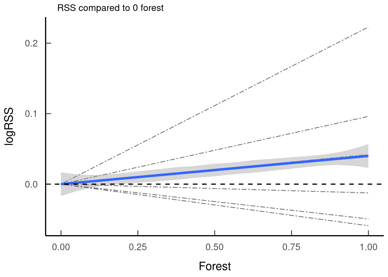
5.2.1.1 Guiding Questions
- If you present individuals and there are drastic differences in their response - can you find a reason for this?
- Take your beta values and interpret them before running your RSS, sketch out a predictive figure for what you would expect the relationships to look like. Do they match up?
- What h values will you choose for your two locations at t2 (x1 and x2)? Will you value h at x2 or ∆h?: look at the distribution of your availability of h and make sure there is biological justification.
- What values do you choose for your interaction? When you are looking at an interaction try to keep your RSSs on a similar scale for easy comparison. If they are wildly different perhaps you should choose less extreme values - again consider biological realism.
5.2.2 Movement
Available steps are drawn from a gamma distribution of step lengths (shape, scale) and a von-Mises distribution of turn angles (kappa, mu)
5.2.2.1 Speed/Step Length
Extract basal parameters:
# sl_distr_params(track)
# ta_distr_params(track)
The calculation for Mean Step Length is shape multiplied by scale:
# > code for this calculation
# > example plot
5.2.2.1.1 Negative Speed Estimates
Negative speed estimates or predictions can come from some models
- First check that your data is ok (clean). Are there some erroneous locations, step lengths, or turn angle? Trust the observed (used) input data.
- Try another step-length distribution
- Include an interaction between step length and turn angle
- Remove ‘non-movement’ steps, short steps below a certain distance. Plot data to determine non-movement behavioural modes
- Resample data to a coarser resolution that has longer steps and less non-movement steps.
How do we calculate speed from an exponential or other distribution?
The shapescale (kappatheta) is the mean expectation of a gamma. The exponential distribution, which is a special case of the gamma, only has a rate parameter (lambda). The mean for the exponential is 1/lambda, so that is how we could get a mean speed from the tentative or modified estimates. The scale parameter is the inverse of rate, for gamma and other distributions. Exponential is a special case where shape = 1, so using a modifier log SL turns it into a gamma. Thus, rate is inverse scale, and shape is one. The equations work out to be the same.
See Julie’s snail code here.
See other distributions in the iSSA webinar files (Avgar and Smith 2022)
5.2.2.2 Directionality
Kappa is the concentration parameter of the von-Mises distribution and indicates directionality (increasing kappa is more forward movement)
5.2.2.2.1 Negative Von Mises Estimates
A negative von Mises concentration parameter means the adjusted turn angle distribution is centred at 𝜋 (180°) rather than 0 (negative directional autocorrelation; behaviourally the animal is more likely to turn back). This can happen with high resolution data. A fix is to multiply by -1 to recenter the distribution and assumption around 0 and not 𝜋.
# > turn angle plot5.3 Model Validation and Evaluation
Often researchers want to determine the performance and reproducibility of their models.
5.3.1 Model Selection
5.3.1.1 AIC/likelihood
It is common to create multiple candidate models and select the top performing one. Performance can be evaluated using a variety of measures, we will discuss some common ones and make our own recommendations.
Competition between candidate models works off a bias-variance trade-off. This trade-off can be superseded by large data sets which then favours complex models. Please read (Fieberg and Johnson 2015, Northrup et al. 2021) for in depth discussion of building and evaluating models.
Likelihood ratios can be used when required.
# > example5.3.2 Model Prediction
5.3.2.1 K-fold ‘Validation’
There are both philosophical and analytical points to be made about validation.
First and foremost, we can’t expect our models to do everything. Some models are built to understand the magnitude of ecological effects and responses, some are built to predict future ecological patterns (regardless of the underlying ecological mechanism). In Habitat Selection Analysis some work is done with the purpose of predicting areas to conserve and identifying important habitat for other populations. Ideally, to test this you would run an HSA, then test it on another population or in a different time period. So, the question was how do we predict and validate models when we don’t have out of sample data? There are many options but k-fold really took hold (Boyce et al. 2002).
In this method you partition the data into ‘k’ number of folds, withhold a fold, run the model and then see how well it predicts the left-out fold. You bin the RSF predictions from the area and rank them, the highest being the most selected, and then take the frequency of used points in each of the bins. The higher your correlation between bin rank and frequency, the better your model
Now, because iSSAs and some other HSAs use conditional logistic regression you can’t make a predictive map easily (but this is coming soon), Instead, an option is to rank within your strata/cluster of used and random points (Fortin et al. 2009). Arguably, this is not ideal because you are restricted to the strata and you actually want a validation of the extent of your study area.
Quinn Webber’s social iSSA repository: https://github.com/qwebber/social-issa/
If the k-fold procedure is used it is critical to mention that as it is done for SSF is not a validation it is an out of sample discrimination test. It is important to accurately state that it is not a predictive validation, this method attempts to discriminate between a used step and an available step.
Two alternative and recommended options are discrimination or habitat calibration.
5.3.2.2 Discrimination analyses
A correct discrimination index for case-control models is concordance (Brentnall et al. 2015). With an r package! https://cran.r-project.org/web/packages/survival/vignettes/concordance.pdf