7 Full workflow

7.1 Preface

This is an example of me (Julie) “talking” the reader through conducting an iSSA on the fisher data that is set up in our targets workflow.

7.2 Preparing an iSSA

7.2.1 The data

The critical data for running an iSSA are the x and y coordinates for GPS relocations and the associated datetime timestamp. Depending on what you’re doing, you’ll probably want to know the individual that those relocations belong to as well.

There are several things that need to be done prior to actually doing an iSSA

Overarchingly:

Clean the GPS data
Prepare the layers and other covariate data

7.2.1.1 Clean the GPS data

Things that you need to check and clean if they are not met:

Make sure all observations (GPS points) are complete

if not, remove incomplete observations

Check if there are duplicated GPS points (two taken at the same time)

remove duplicate observations

7.2.1.2 Prepare covariate input data

It is critical that all of the layers you plan to use and GPS points are in the same coordinate reference system. This can take a long time to reproject layers, crop them, and anything else you need to do for everything to be in the same “world,” but it is critical to do for the later steps of extracting covariates by step.

7.2.2 Making tracks

Once the data is clean, we make the points into a track. If you have more than one individual in the dataset, do it by individual.

Generating tracks:

make_track(locs_prep, x_, y_, t_, all_cols = TRUE, crs = epsg)

7.2.2.1 Check the sampling rate

Now we should check how the sampling rate looks due to the messiness of GPS relocations.

summarize_sampling_rate_many(tar_read(tracks), 'id')

id	min	q1	median	mean	q3	max	sd	n	unit
1072	3.92	9.8	10.0	20.7	10.3	1650	95	1348	min
1465	0.40	2.0	2.0	8.9	4.0	1080	48	3003	min
1466	0.42	2.0	2.1	15.7	4.1	2167	104	1500	min
1078	1.35	9.8	10.0	21.7	10.3	2111	87	1637	min
1469	0.42	2.0	2.2	13.2	5.4	2889	90	2435	min
1016	0.07	1.9	2.0	8.0	2.5	1209	44	8957	min

Data are messy. For iSSA, we need the GPS fixes to happen at regular intervals, the same for all individuals in the model, so we likely need to resample the data.

resample_tracks(tracks, rate = rate, tolerance = tolerance)

In our targets workflow, we have simplified all of this. Here, all you will have to do is at the beginning of the workflow: fill in the Variables to match your data.

# Variables ---------------------------------------------------------------
# Targets: prepare
id_col <- 'id'
datetime_col <- 't_'
x_col <- 'x_'
y_col <- 'y_'
epsg <- 32618
crs <- st_crs(epsg)
crs_sp <- CRS(crs$wkt)
tz <- 'America/New_York'

# Targets: tracks
# Split by: within which column or set of columns (eg. c(id, yr))
#  do we want to split our analysis?
split_by <- id_col

# Resampling rate
rate <- minutes(30)

# Tolerance
tolerance <- minutes(5)

# Number of random steps
n_random_steps <- 10

7.2.3 Steps

Now we have tracks, but a step selection analysis requires steps! So, in our targets workflow, we only keep data for individuals that have at least 3 steps, and this is adjustable depending on what you need.

7.2.3.1 Check the distribution of steps and turn angles

Now to make sure there aren’t any biological impossibilities in the steps. Usually there are a lot of little steps and few big steps, but this is a good check to make sure any erroneous observations are removed. For instance, this would show if there are any steps that are not biologically possible. It also shows the distribution so you know if you should use a Gamma or exponential distribution for generating random steps. Most are Gamma, and that is the default in amt.

SL distribution for 1 individual

tar_read(dist_sl_plots, 1)

## $dist_sl_plots_8ba21cb0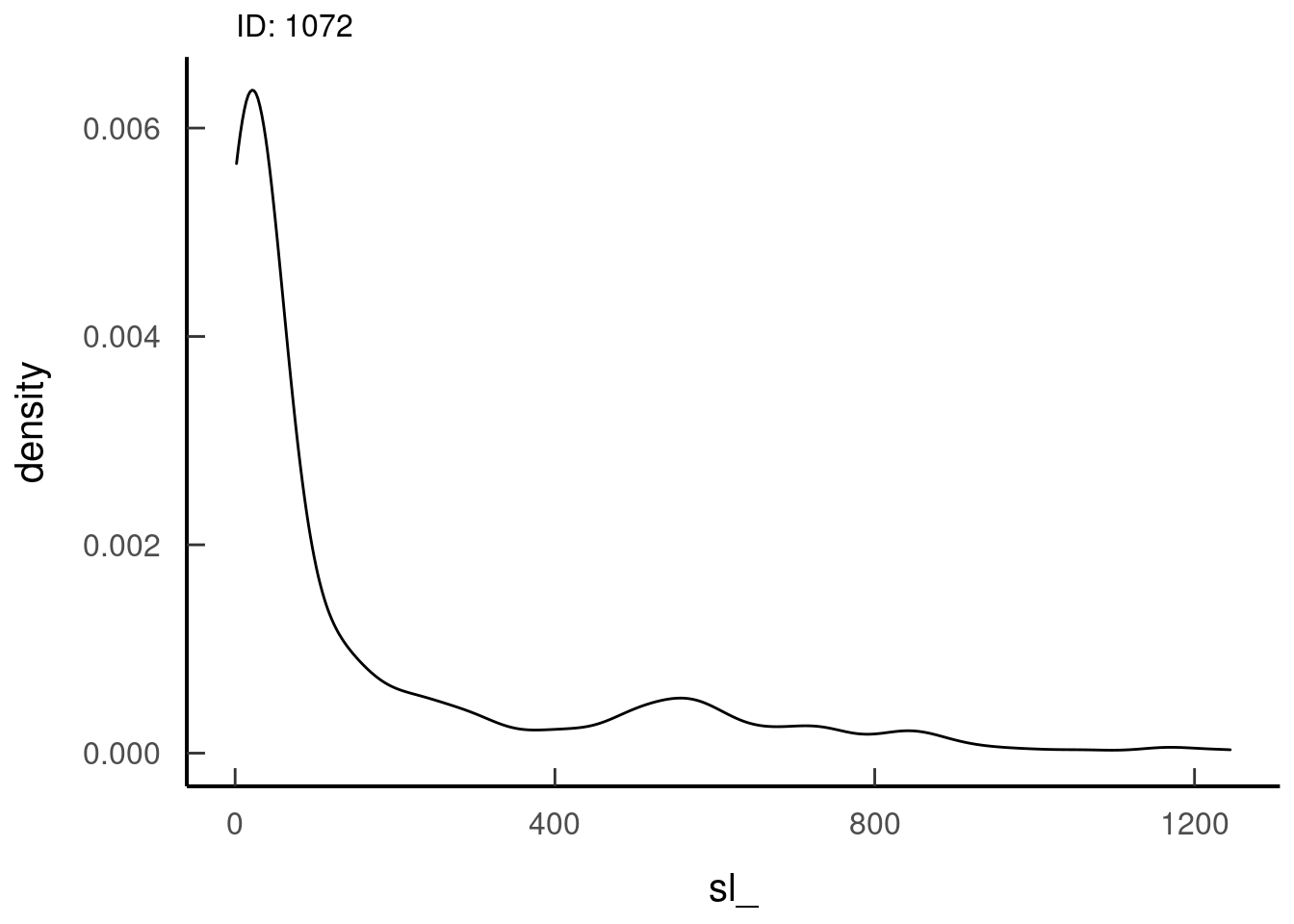

Looks like a gamma distribution, so that’s good

TA distribution for 1 individual

tar_read(dist_ta_plots, 1)

## $dist_ta_plots_8ba21cb0

## Warning: Removed 35 rows containing non-finite values (stat_density).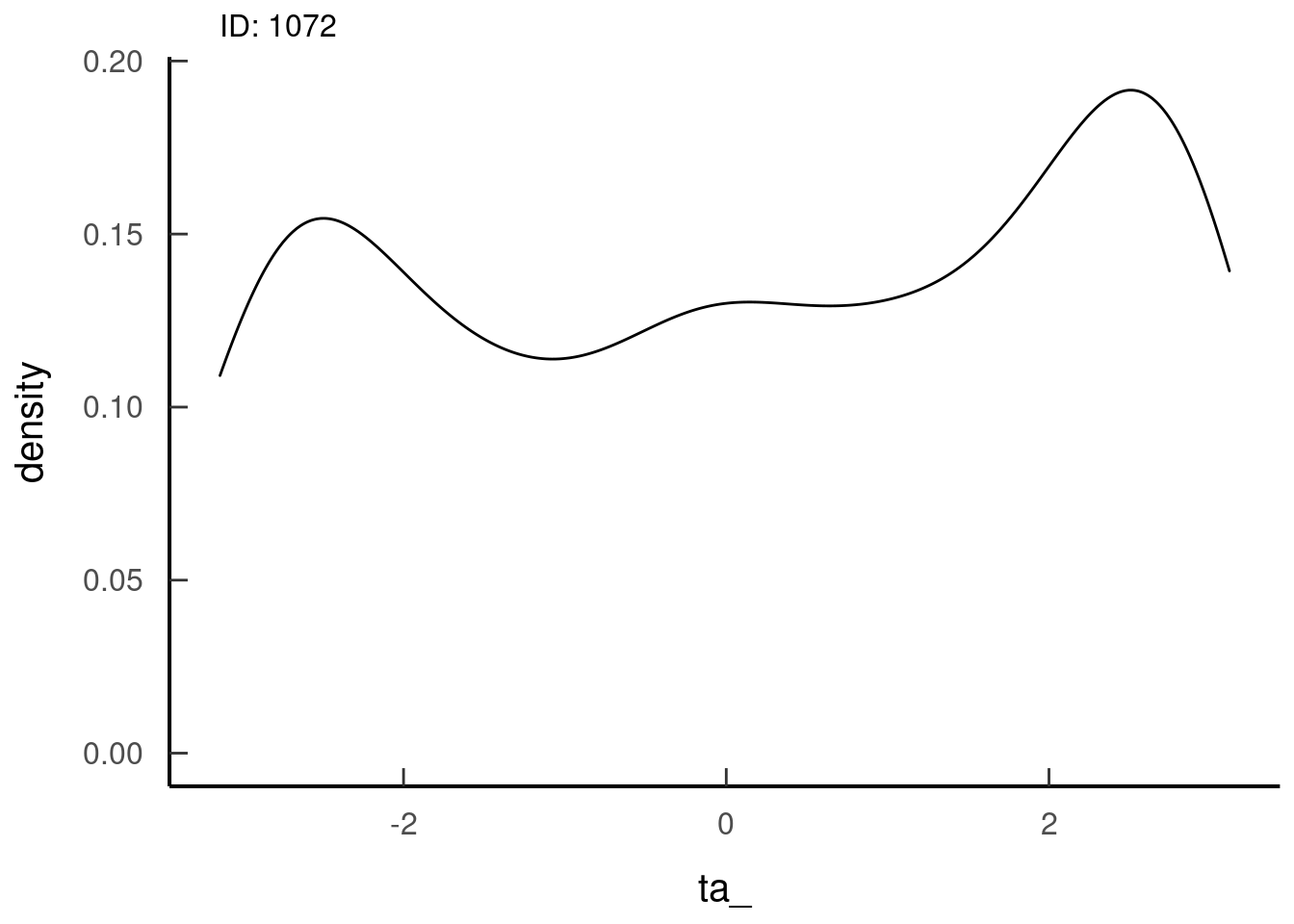

Looks like a von Mises distribution, so that’s also good

7.2.4 Prepare the data to go into the iSSA

So, at this point, we have our observed steps and know what their distributions look like. Now we can use this information to properly inform our random steps with the correct distribution. As we create the random steps, we will also extract the covariates of interest at each step.

7.2.4.1 Motivation vs Selection

One of the critical decisions to make in your analysis is if you want to know if a variable is motivating why/how an animal moves vs. if the animal is selecting for that variable; this decision influences if you use the information from the start of the step (motivation) vs. the end of the step (selection) in your analysis. This decision is of course determined by your question and hypotheses

See Choosing covariates for more info

7.2.4.2 Example extraction

For example, here we are creating random steps and extracting information about what landcover class and the distance from water an individual selects (at the end of each step) and time of day (day or night at the start of the step) at the time of each step. This will create a dataset that includes step length, turn angle, whether it’s day or night at the start of the step, and what land class an animal is on at the end of their step.

NOTE: In the targets workflow, we have created out own extraction functions instead of using amt’s extract_covariate and time_of_day functions. This is for several reasons - more flexibility - amt isn’t functional with terra yet (coming soon) - time_of_day is good for day vs night, but if you want dawn or dusk, it’s not great at larger fixrates. For instance, if you have a 2 hour fixrate, it rarely includes dawn or dusk because those time frames are narrow in the default maptools function that time_of_day wraps around. In this circumstance, we have created our own time of day extractions as needed by location. However, for our fisher example here with a 30 minute fixrate, including default crepuscular times should be fine.

# R/extract_layers.R
extract_layers

function (DT, crs, lc, legend, elev, popdens, water) 
{
    setDT(DT)
    start <- c("x1_", "y1_")
    end <- c("x2_", "y2_")
    extract_pt(DT, lc, end)
    DT[legend, `:=`(lc_description, description), on = .(pt_lc = Value)]
    extract_pt(DT, elev, end)
    extract_pt(DT, popdens, end)
    extract_distance_to(DT, water, end, crs)
}

If you have multiple hypotheses that would benefit from know information from both the beginning and the end of the step, you can input"both" instead of "start" or "end".

So, in the end, we get a dataset that looks something like:

x1_	x2_	y1_	y2_	sl_	ta_	id	tar_group	burst_	t1_	t2_	dt_	step_id_	case_	pt_lc	lc_description	pt_elev	pt_popdens	dist_to_water
593975	593969	4739337	4739492	155.61	NA	1072	1	4	2011-02-13 04:31:32	2011-02-13 05:00:13	29 mins	1	TRUE	41	forest	83	51	171
593975	593967	4739337	4739367	31.62	0.21	1072	1	4	2011-02-13 04:31:32	2011-02-13 05:00:13	29 mins	1	FALSE	42	forest	100	102	289
593975	593959	4739337	4739362	29.55	0.52	1072	1	4	2011-02-13 04:31:32	2011-02-13 05:00:13	29 mins	1	FALSE	42	forest	100	102	297
593975	594216	4739337	4739595	353.46	-0.79	1072	1	4	2011-02-13 04:31:32	2011-02-13 05:00:13	29 mins	1	FALSE	21	developed	58	51	49
593975	593973	4739337	4739338	2.03	0.90	1072	1	4	2011-02-13 04:31:32	2011-02-13 05:00:13	29 mins	1	FALSE	42	forest	105	102	314
593975	594090	4739337	4739452	162.43	-0.83	1072	1	4	2011-02-13 04:31:32	2011-02-13 05:00:13	29 mins	1	FALSE	41	forest	77	51	180
593975	593978	4739337	4739339	4.15	-0.93	1072	1	4	2011-02-13 04:31:32	2011-02-13 05:00:13	29 mins	1	FALSE	42	forest	105	102	311
593975	593829	4739337	4739372	150.09	1.29	1072	1	4	2011-02-13 04:31:32	2011-02-13 05:00:13	29 mins	1	FALSE	43	forest	90	102	333
593975	593916	4739337	4739366	66.11	1.06	1072	1	4	2011-02-13 04:31:32	2011-02-13 05:00:13	29 mins	1	FALSE	43	forest	97	102	305
593975	593975	4739337	4739337	0.48	1.41	1072	1	4	2011-02-13 04:31:32	2011-02-13 05:00:13	29 mins	1	FALSE	42	forest	105	102	314
593975	594066	4739337	4739605	283.09	-0.37	1072	1	4	2011-02-13 04:31:32	2011-02-13 05:00:13	29 mins	1	FALSE	41	forest	72	51	32

7.3 Running an iSSA

This workflow is going to be an example using the Poisson point process method described by Muff et al (2020). This method allows us to look at all individuals at once so we can examine both the individual- and population-level responses at once. In this example, we’re going to include both categorical and continuous variables.

NOTE: Random effects in GLMMs are supposed to have 5 or more levels, which means you should have at least 5 individuals if you want to include them as a random effect.

# R/model_land_cover.R
model_land_cover

function (DT) 
{
    glmmTMB(case_ ~ -1 + I(log(sl_)) + I(log(sl_)):lc_adj + lc_adj + 
        I(log(dist_to_water + 1)) + I(log(dist_to_water + 1)):I(log(sl_)) + 
        (1 | indiv_step_id) + (0 + I(log(sl_)) | id) + (0 + I(log(sl_)):lc_adj | 
        id) + (0 + lc_adj | id) + (0 + I(log(dist_to_water + 
        1)) | id) + (0 + I(log(dist_to_water + 1)):I(log(sl_)) | 
        id), data = DT, family = poisson(), map = list(theta = factor(c(NA, 
        1:23))), start = list(theta = c(log(1000), seq(0, 0, 
        length.out = 23))))
}

summary(tar_read(model_lc))

##  Family: poisson  ( log )
## Formula:          
## case_ ~ -1 + I(log(sl_)) + I(log(sl_)):lc_adj + lc_adj + I(log(dist_to_water +  
##     1)) + I(log(dist_to_water + 1)):I(log(sl_)) + (1 | indiv_step_id) +  
##     (0 + I(log(sl_)) | id) + (0 + I(log(sl_)):lc_adj | id) +  
##     (0 + lc_adj | id) + (0 + I(log(dist_to_water + 1)) | id) +  
##     (0 + I(log(dist_to_water + 1)):I(log(sl_)) | id)
## Data: DT
## 
##      AIC      BIC   logLik deviance df.resid 
##       NA       NA       NA       NA    26488 
## 
## Random effects:
## 
## Conditional model:
##  Groups        Name                                  Variance Std.Dev. Corr 
##  indiv_step_id (Intercept)                           1.00e+06 1.00e+03      
##  id            I(log(sl_))                           1.87e-90 1.37e-45      
##  id.1          I(log(sl_)):lc_adjdisturbed           1.08e-02 1.04e-01      
##                I(log(sl_)):lc_adjforest              2.05e-03 4.52e-02 -1.00
##                I(log(sl_)):lc_adjopen                1.08e-01 3.28e-01  1.00
##                I(log(sl_)):lc_adjwetlands            2.05e-03 4.53e-02 -1.00
##  id.2          lc_adjdisturbed                       4.42e-01 6.64e-01      
##                lc_adjforest                          3.32e-02 1.82e-01 -1.00
##                lc_adjopen                            4.42e+00 2.10e+00  1.00
##                lc_adjwetlands                        2.38e-26 1.54e-13 -0.27
##  id.3          I(log(dist_to_water + 1))             1.34e-02 1.16e-01      
##  id.4          I(log(dist_to_water + 1)):I(log(sl_)) 5.26e-90 2.29e-45      
##              
##              
##              
##              
##              
##  -1.00       
##   1.00 -1.00 
##              
##              
##  -1.00       
##   0.30 -0.28 
##              
##              
## Number of obs: 26521, groups:  indiv_step_id, 2411; id, 6
## 
## Conditional model:
##                                       Estimate Std. Error z value Pr(>|z|)
## I(log(sl_))                           -0.13107        NaN     NaN      NaN
## lc_adjdisturbed                       -3.74565        NaN     NaN      NaN
## lc_adjforest                          -3.42646        NaN     NaN      NaN
## lc_adjopen                            -5.94910        NaN     NaN      NaN
## lc_adjwetlands                        -3.67823        NaN     NaN      NaN
## I(log(dist_to_water + 1))             -0.03581        NaN     NaN      NaN
## I(log(sl_)):lc_adjforest               0.23726        NaN     NaN      NaN
## I(log(sl_)):lc_adjopen                 0.29305        NaN     NaN      NaN
## I(log(sl_)):lc_adjwetlands             0.28385        NaN     NaN      NaN
## I(log(sl_)):I(log(dist_to_water + 1))  0.00072        NaN     NaN      NaN

When looking at the output of this model, we see some issues. First of all, there are some warnings from the model. The positive hessian warning is applied liberally in glmmTMB, but the real sign of a problem is the NAs reported for variation. This model didn’t converge properly, so we need to look at why.

Things to explore at the data level include:

lots of NAs for a particular variable (helpful tips from Bolker)
lots of variation or very little variation in a particular variable
availability of variables for individuals

Things to explore at the model level include:

the model is over-parameterized for the amount of data
the high variance is assigned at the strata level and not for another random effect
variables are similarly scaled
if using the Muff method, the strata represent the step id by individual (indiv_step_id), not the step id that is assigned by amt because the way we have it coded, the numbers restart for each individual
categorical variables are classified as factors, especially indiv_step_id
random effects have at least 5 levels (this is likely not going to be a problem for most iSSAs, but it has come up)

# checking availability 
# for landcover
tar_read(avail_lc)

id	prop_lc_description	lc_description
1072	0.72	forest
1072	0.16	developed
1072	0.01	water
1072	0.02	cultivated
1072	0.07	wetlands
1072	0.00	barren
1072	0.00	shrubland
1465	0.37	wetlands
1465	0.19	developed
1465	0.37	forest
1465	0.07	cultivated
1465	0.01	barren
1465	0.00	water
1465	0.00	shrubland
1466	0.61	wetlands
1466	0.17	developed
1466	0.05	cultivated
1466	0.15	forest
1466	0.01	water
1078	0.48	forest
1078	0.28	developed
1078	0.21	wetlands
1078	0.00	shrubland
1078	0.03	cultivated
1078	0.00	water
1469	0.18	forest
1469	0.06	cultivated
1469	0.42	developed
1469	0.33	wetlands
1469	0.01	water
1016	0.49	forest
1016	0.16	developed
1016	0.01	shrubland
1016	0.20	wetlands
1016	0.06	cultivated
1016	0.08	water
1016	0.00	herbaceous

# for distance to water
tracks_extract <- tar_read(tracks_extract)
tracks_extract[!(case_), quantile(dist_to_water, na.rm = TRUE), by = id]

id	V1
1072	0
1072	285
1072	1131
1072	1714
1072	3049
1465	0
1465	595
1465	854
1465	1188
1465	2573
1466	0
1466	222
1466	418
1466	809
1466	2154
1078	0
1078	1833
1078	2271
1078	2604
1078	3376
1469	0
1469	418
1469	791
1469	1365
1469	2594
1016	0
1016	135
1016	442
1016	918
1016	1839

After some exploration, I’m thinking this model is over-parameterized for 6 individuals, at least having so many landcover classes. So, I’m going to pretend for this example that we only care about selection for forest and disturbed habitats. We created dummy variables for this based on the extracted landcover data and ran the iSSA on this data.

# R/model_forest_bin.R
model_forest_bin

function (DT) 
{
    glmmTMB(case_ ~ -1 + I(log(sl_)) + I(log(sl_)):forest + forest + 
        I(log(sl_)):disturbed + disturbed + I(log(dist_to_water + 
        1)) + I(log(dist_to_water + 1)):I(log(sl_)) + (1 | indiv_step_id) + 
        (0 + I(log(sl_)) | id) + (0 + I(log(sl_)):disturbed | 
        id) + (0 + I(log(sl_)):forest | id) + (0 + forest | id) + 
        (0 + disturbed | id) + (0 + I(log(dist_to_water + 1)) | 
        id) + (0 + I(log(dist_to_water + 1)):I(log(sl_)) | id), 
        data = DT, family = poisson(), map = list(theta = factor(c(NA, 
            1:7))), start = list(theta = c(log(1000), seq(0, 
            0, length.out = 7))))
}

summary(tar_read(model_forest))

##  Family: poisson  ( log )
## Formula:          
## case_ ~ -1 + I(log(sl_)) + I(log(sl_)):forest + forest + I(log(sl_)):disturbed +  
##     disturbed + I(log(dist_to_water + 1)) + I(log(dist_to_water +  
##     1)):I(log(sl_)) + (1 | indiv_step_id) + (0 + I(log(sl_)) |  
##     id) + (0 + I(log(sl_)):disturbed | id) + (0 + I(log(sl_)):forest |  
##     id) + (0 + forest | id) + (0 + disturbed | id) + (0 + I(log(dist_to_water +  
##     1)) | id) + (0 + I(log(dist_to_water + 1)):I(log(sl_)) |      id)
## Data: DT
## 
##      AIC      BIC   logLik deviance df.resid 
##    49162    49276   -24567    49134    26507 
## 
## Random effects:
## 
## Conditional model:
##  Groups        Name                                  Variance Std.Dev.
##  indiv_step_id (Intercept)                           1.00e+06 1.00e+03
##  id            I(log(sl_))                           1.26e-09 3.55e-05
##  id.1          I(log(sl_)):disturbed                 7.67e-04 2.77e-02
##  id.2          I(log(sl_)):forest                    2.65e-10 1.63e-05
##  id.3          forest                                1.77e-02 1.33e-01
##  id.4          disturbed                             1.23e-10 1.11e-05
##  id.5          I(log(dist_to_water + 1))             1.34e-02 1.16e-01
##  id.6          I(log(dist_to_water + 1)):I(log(sl_)) 1.55e-11 3.93e-06
## Number of obs: 26521, groups:  indiv_step_id, 2411; id, 6
## 
## Conditional model:
##                                       Estimate Std. Error z value Pr(>|z|)    
## I(log(sl_))                            0.07923    0.07735    1.02    0.306    
## forest                                 0.34653    0.19410    1.79    0.074 .  
## disturbed                             -0.19495    0.27753   -0.70    0.482    
## I(log(dist_to_water + 1))              0.08271    0.08956    0.92    0.356    
## I(log(sl_)):forest                    -0.05632    0.03635   -1.55    0.121    
## I(log(sl_)):disturbed                 -0.24794    0.05330   -4.65  3.3e-06 ***
## I(log(sl_)):I(log(dist_to_water + 1))  0.00875    0.01142    0.77    0.444    
## ---
## Signif. codes:  0 '***' 0.001 '**' 0.01 '*' 0.05 '.' 0.1 ' ' 1

This model runs without issue.

7.4 Interpretation

Demonstrating effects from iSSA output is an area where you will see a lot of different avenues at this point. Some just show the beta estimates from the model and p-values. This, however can result in misinterpretation of biological significance (Avgar et al. 2017).

7.4.1 Relative Selection Strength

This is where Relative Selection Strength (RSS) comes in. Avgar et al (2017) derived various equations to calculate RSS depending on if variables are on their own, interacted with others, log-transformed, etc. However, since then Brian Smith has determined that using the predict() function can achieve the same outcome (see proof Smith 2020). But this is all the mathematical details. What RSSs are really doing is comparing the selection strength for habitat at location 1 (H1) compared to location 2 (H2).So, say an animal is not in a forest, are they relatively more likely to select to be in a forest or avoid the forest? Then the RSS shows the strength of selection or avoidance over a range of habitat values of that habitat type.

In the targets-issa workflow, we predict H1, and H2 for forest using the following functions:

# R/predict_h1_forest.R
predict_h1_forest

## function (DT, model) 
## {
##     N <- 100L
##     new_data <- DT[, .(sl_ = mean(sl_), forest = seq(from = 0, 
##         to = 1, length.out = N), disturbed = 0, dist_to_water = median(dist_to_water, 
##         na.rm = TRUE), indiv_step_id = NA), by = id]
##     new_data[, `:=`(h1_forest, predict(model, .SD, type = "link", 
##         re.form = NULL))]
##     new_data[, `:=`(x, seq(from = 0, to = 1, length.out = N)), 
##         by = id]
## }

# R/predict_h2.R
predict_h2

## function (DT, model) 
## {
##     new_data <- DT[, .(sl_ = mean(sl_), forest = 0, disturbed = 0, 
##         dist_to_water = median(dist_to_water, na.rm = TRUE), 
##         indiv_step_id = NA), by = id]
##     new_data[, `:=`(h2, predict(model, .SD, type = "link", re.form = NULL))]
## }

# Then we can calculate RSS for forest as H1 - H2:

# R/calc_rss.R
calc_rss

## function (pred_h1, h1_col, pred_h2, h2_col) 
## {
##     log_rss <- merge(pred_h1[, .SD, .SDcols = c("id", "x", h1_col)], 
##         pred_h2[, .SD, .SDcols = c("id", h2_col)], by = "id", 
##         all.x = TRUE)
##     log_rss[, `:=`(rss, h1 - h2), env = list(h1 = h1_col, h2 = h2_col)]
## }

And finally, the plots with the plot_rss function.

tar_read(plot_rss_forest)

## `geom_smooth()` using method = 'loess' and formula 'y ~ x'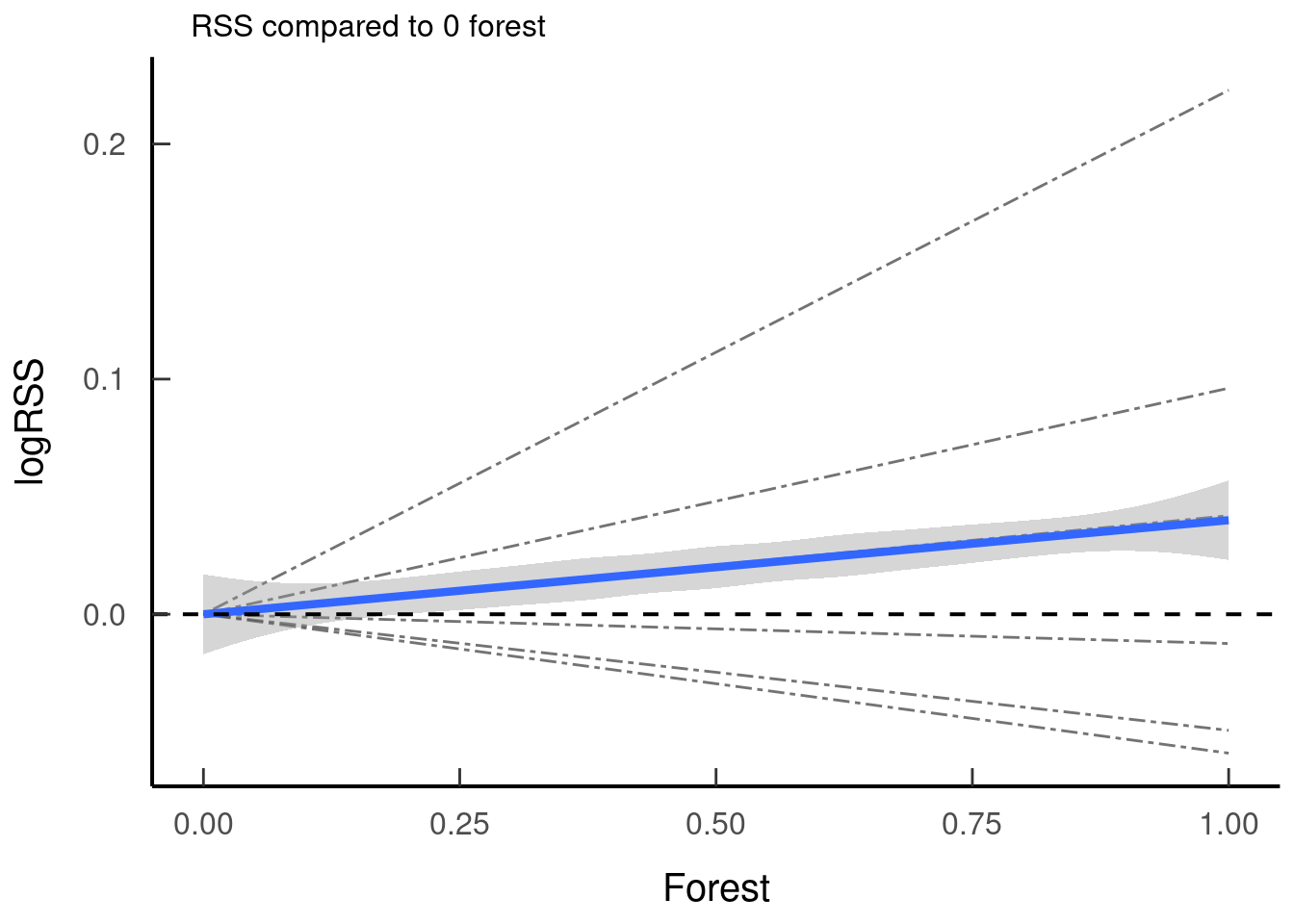

JWT comment: I personally find it hard to wrap my head around RSSs for categorical variables, and I don’t have a great way of explaining it for others like me who didn’t get it. The closest I can describe is, say, looking at this plot, the individual starts not in forest, is their next step more likely to go to forest or not. To continuous nature of the RSS is hard for me to wrap my head around with a categorical variable. I just pretend in my head that it’s a proportional value of ‘no forest’ = 0 and ‘all forest’ = 1, and the middle is an estimate based on the model. It’s not perfect, but that’s the best I’ve been able to come to terms with it. :shrug: #OverlyHonestMethods

We can then do the same thing to determine the RSS for distance to water.

tar_read(plot_rss_water)

## `geom_smooth()` using method = 'loess' and formula 'y ~ x'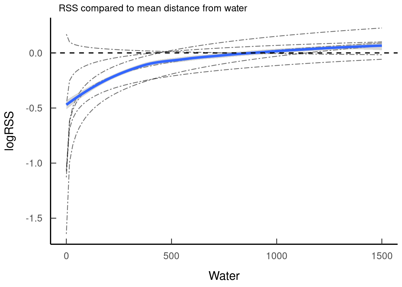

RSSs have to be done one habitat at a time. That being said, interactions can be explored by pre-determining cut off points to examine one of the variables at a time. I know that sounds confusing. So, for example, we have selection of forest interacted with distance to road. Say we want to understand how animals select for forest when they are near or far from roads. So, we define being near a road as being 100m of the road and being far from the road as 5000m from the road. These values are semi-arbitrary, but they should be based on the biology of the animal. This complicates the calculation of the RSS a bit, making it a two step process with the predict method. You first have to calculate the overall selection for, in this case, forest at 100m from the road, then you run the run the predict function over the availability of forest and add them together.

7.4.2 Speed

Speed is a different kettle of fish. Some people show box plots of step length to give an idea of speed, but this is only a partial show of effect size (this is not phrased well – fix). When using a gamma distribution for an iSSA, the mean estimated speed is shape parameter multiplied by the scale parameter from the gamma distribution. However, the shape is modified by the movement variables in the iSSA itself. So this calculation becomes

\(\text{mean estimated speed} = (shape + logSL.beta + logSLintx.beta*mean(what.interacted.with))*scale\)

So, from our toy example, this could be done as below. Here, we can pick which covariate we want to vary to estimate speed to see how speed is impacted by what it is interacted with. seq represents the range of values we’re looking over.

# R/calc_speed.R
calc_speed

## function (DT, covariate, seq) 
## {
##     if (covariate == "forest") 
##         DT[, `:=`(spd = list(list((shape + `I(log(sl_))` + `I(log(sl_)):forest` * 
##             seq + `I(log(sl_)):disturbed` + `I(log(dist_to_water + 1)):I(log(sl_))` * 
##             median.water) * (scale))), x = list(list(seq))), 
##             by = .(id)]
##     if (covariate == "disturbed") 
##         DT[, `:=`(spd = list(list((shape + `I(log(sl_))` + `I(log(sl_)):forest` + 
##             `I(log(sl_)):disturbed` * seq + `I(log(dist_to_water + 1)):I(log(sl_))` * 
##             median.water) * (scale))), x = list(list(seq))), 
##             by = .(id)]
##     if (covariate == "dist_to_water") 
##         DT[, `:=`(spd = list(list((shape + `I(log(sl_))` + `I(log(sl_)):forest` + 
##             `I(log(sl_)):disturbed` + `I(log(dist_to_water + 1)):I(log(sl_))` * 
##             seq) * (scale))), x = list(list(seq))), by = .(id)]
##     move <- DT[, .(spd = unlist(spd), x = unlist(x)), by = .(id)]
##     move
## }

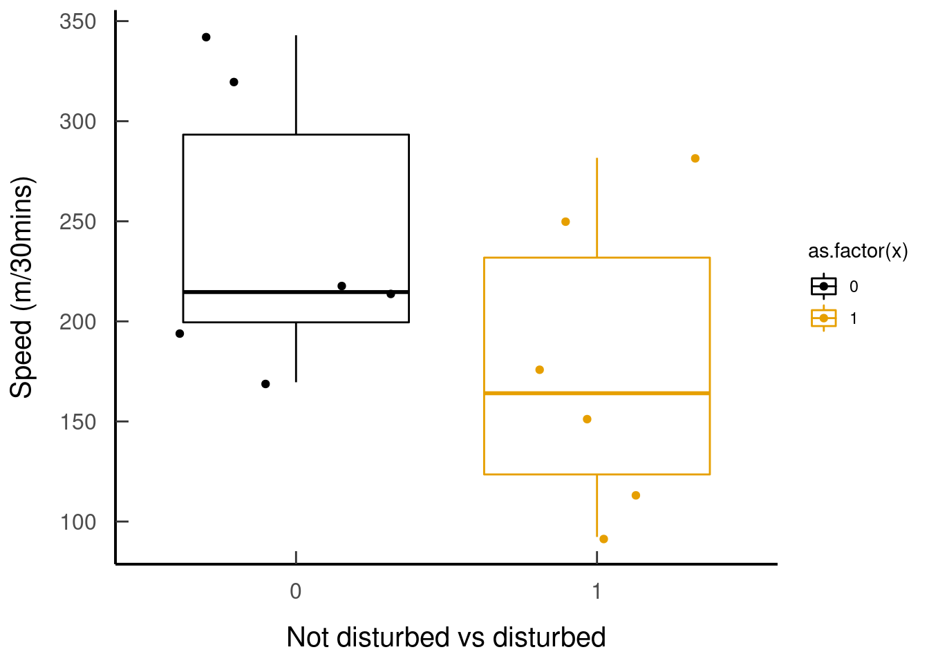
Let’s see how fishers’ speed changes in areas without anthropogenic disturbance vs areas that are disturbed (seq = 0:1)

tar_read(plot_speed_disturbed)

6 Resources

References